Steel Grinding (LAI)

The task in the steel grinding domain is to determine the roughness of the workpiece from the properties of the sound produced during the process of steel grinding. The broader aim of the study was to elaborate the results from the point of view of machine control, where the task is to perform relevant control actions in response to parameter values monitored during the process execution. Since control action is easily deducible from workpiece roughness, the subproblem of workpiece roughness estimation was addressed first. Several machine learning techniques were already applied to the problem, yielding encouraging results (Filipic et al. 1991).

Application domain:	Steel Grinding
Further specification:	Data set
Pointers:	Contact Aram Karalic Aram.Karalic@ijs.si
Data complexity:	123 examples
Data format:	Prolog

FORS Experiments

Data were obtained during an experiment in which vibration signals generated by the grinding wheel and the workpiece were detected by an accelerometer sensor and processed by a spectrum analyzer (Junkar et al. 1991). From the obtained spectra predefined spectral features were extracted: total spectrum area (SpArea), frequency of the maximum area peak (MaxAreaX), and frequency of the spectrum area central point (AreaCX). Simultaneously, workpiece surface roughness was measured.

Two background knowledge literals were defined: =< and >=, enabling FORS to compare the frequencies.

Expert's Evaluation and Conclusions

It turned out that the use of background knowledge did not bring any significant improvement in the model quality in terms of RE. However, the newly induced models frequently contained background knowledge literals. The domain experts considered this a significant improvement because newly induced models are more general than the models without background knowledge. For example, without using background knowledge, a literal such as MaxAreaX <= 6125 typically appeared, saying that the frequency of the maximum area peak is less than 6125Hz. In this particular setting (grinding regime, choice of the tools) this means that the maximum area peak is in the lower part of the spectrum. Using different grinding wheel speed the whole spectrum would shift to higher or lower frequencies, thus making the above literal useless. However, usage of background knowledge typically yielded literal MaxAreaX <= AreaCX, which directly states that the maximum peak must lie in the lower part of the spectrum, regardless of the frequency area in which the spectrum is situated, therefore enabling rule usage in much broader class of working regimes.

The model using linear regression constructed from all examples by using MDL pruning was chosen for closer inspection:

    f(Roughness,SpArea,MaxAreaX,AreaCX) :-
        AreaCX =< 5600, MaxAreaX <= AreaCX,
        SpArea =< 0.25, Roughness is 1.70,!.
    f(Roughness,SpArea,MaxAreaX,AreaCX) :-
        MaxAreaX <= AreaCX, AreaCX =< 5890,
        MaxAreaX =< 1140,
        Roughness is 0.00169 * MaxAreaX,!.
    f(Roughness,SpArea,MaxAreaX,AreaCX) :-
        AreaCX >= 7310, SpArea >= 0.2130,
        Roughness is 0.00016832 * AreaCX,!.
    f(Roughness,SpArea,MaxAreaX,AreaCX) :-
        MaxAreaX <= AreaCX, SpArea >= 0.33,
        AreaCX >= 5950,
        Roughness is 0.00029 * AreaCX,!.
    f(Roughness,SpArea,MaxAreaX,AreaCX) :-
        SpArea =< 0.1700, Roughness is 0.98,!.
    f(Roughness,SpArea,MaxAreaX,AreaCX) :-
        AreaCX =< 5890, Roughness is 1.72,!.
    f(Roughness,SpArea,MaxAreaX,AreaCX) :-
        SpArea =< 0.23,
        Roughness is 5.4102 * SpArea,!.
    f(Roughness,SpArea,MaxAreaX,AreaCX) :-
        SpArea >= 0.31, AreaCX >= 6190,
        Roughness is 1.38,!.
    f(Roughness,SpArea,MaxAreaX,AreaCX) :-
        MaxAreaX >= 5730, SpArea >= 0.33,
        Roughness is 4.13661194 * SpArea,!.
    f(Roughness,SpArea,MaxAreaX,AreaCX) :-
        AreaCX <= MaxAreaX, Roughness is 1.28,!.
    f(Roughness,SpArea,MaxAreaX,AreaCX) :-
        Roughness is 1.82,!.

Expert's evaluation of the model follows:

The condition of the first clause has three parts. The first part selects low frequency of the spectrum central point, that is, small average number of cutting particles. At a simultaneous requirement for a frequency of the central point to be larger than the frequency of the maximum peak it also confines the frequency of the maximum peak to be at least 1140Hz. This yields rather large roughness which means that low frequencies of the maximum area peak imply large roughness. This indicates that roughness is determined by the largest particles, since even relatively small number of such particles can easy spoil the surface.
Second clause confines the frequency of the area central point to the narrow interval between 5600Hz and 5890Hz and with the other part of the condition equal to the first condition, estimates roughness as a linear function of the maximum peak frequency. The clause excellently describes a group of data points near the largest frequency 1100Hz (Figure 1). This clause is also consistent with the first two models, except that the roughness is this time described as a function.
Clause number 3 tells us that high frequency of the area central point and small spectrum area imply low roughness. The following rule is clearly revealed: a large average number of cutting particles (small particles) and low spectrum area imply low roughness.
Clause 4 describes a group of measurements with low highest frequencies of the spectrum. In spite of high frequency of the spectrum area central point (one would then expect small roughness), we get, at the simultaneous high spectrum area ( the power), a large roughness. The roughness in this situation linearly increases with the frequency of the area central point. This clause again states that a small number of large particles can significantly spoil the surface.
Clause five tells us that the roughness is low when the power of the process is low, independently of the size of the particles.
Clause six again confirms the fact that the largest particles determine the quality of the surface. Small average number of cutting particles implies bad surface.
Clauses 7, 8, and 9 split the parameter space according to the spectrum area and assign each subspace a linear relationship between the roughness and the spectrum area, thus confirming the fact that larger cutting power implies bad surface.

0.8mm

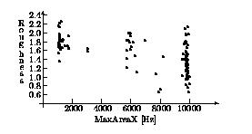
Figure 1: Roughness vs. frequency of the maximum area peak (MaxAreaX) in the domain of steel grinding. Domain expert claims to be satisfied with the results of machine learning since our models enabled him to grasp some additional process properties which he wouldn't be able to discover only with classical statistical tools. However, he suggests that the machine learning approach should not be used alone but should be considered as a powerful supplement to the already existent instruments. It is also worth noting that if the expert had to choose between two equally good models in terms of RE, he usually chose the larger model, justifying the decision by stating that the smaller model does not grasp sufficient detail. However, when choosing amongst the models which had 1, 2 or 3 variables in linear regression terms, he chose the model with only one variable in linear regression terms claiming that it is easier to understand. He also preferred such models over the models with no linear regression.

References

Bogdan Filipic, Miha Junkar, Ivan Bratko, and Aram Karalic. An application of machine learning to a metal-working process. In Proceedings of ITI-91, pages 167-172, Cavtat, Croatia, 1991.
Miha Junkar, Bogdan Filipic, and Ivan Bratko. Identifying the grinding process by means of inductive machine learning. In Preprints of the first CIRP Workshop on Intelligent Manufacturing Systems, Budapest, Hungary, 1991.
A. Karalic, I. Komel, R. Posel. Applications of artificial intelligence in mechanical engineering. In B. Zajc, F. Solina (eds.) Proceedings of the Fifth Electrotechnical and Computer Science Conference, ERK'96, (Portoroz, Slovenia, September 1996), B:175-178. 1996.

back to index