Modeling algal growth in the Lake of Bled (LAI)

The task was to model algal biomass quantity in the Lake of Bled, Slovenia. Eutrophication of the Lake of Bled progressed in big steps this century, endangering the tourist economy of the region. Several restoration measures have been undertaken to avoid the disturbing algal blooms (Kompare and Rismal 1992). Modeling of the algal biomass quantity could help understanding the mechanisms which influence the algal blooms and choosing the measures to prevent them.

Application domain:	Modeling algal growth in the Lake of Bled
Further specification:	Data sets
Pointers:	Contact Aram Karalic Aram.Karalic@ijs.si
Data complexity:	Eight data sets of approx. 60 examples each
Data format:	Prolog

Measurements were provided by the National Institute of Biology, University of Ljubljana. During six years (1987-1992) several quantities were measured in approximately monthly intervals. The measured quantities, used as attributes in the learning process, include:

• Bio ... algal biomass [mg/l],
• NH₄ ... ammonia [mg/l],
• NO₂ ... nitrite [mg/l],
• NO₃ ... nitrate [mg/l],
• OrtP ... orthophosphate PO [mg/l],
• P_tot ... total phosphorus [mg/l],
• Si ... silicon [mg/l],
• TEMP ... temperature,
• Month

The measurements were taken at 2m depth intervals. The results were then grouped to describe a situation in three water layers -- epilimnion (top-most layer, depth from 0m to 4-8m), metalimnion (8m to 12m) and hypolimnion, which consisted of the rest of the water. For every layer, two ways of combining the measurements within the layer were employed:

• averaging the data points,
• finding a data point with the maximal value.

Additionally we took into account the fact, that the lake is naturally divided in two basins -- east and west basin.

We decided not to make any experiments concerning the hypolimnion, since we were concerned primarily with modeling of biomass which appears mainly in the upper two layers.

So, we were actually faced with 8 subproblems:
 

FORS Experiments

Eight kinds of models for biomass prediction were induced, predicting average and maximal values, values for epilimnion and metalimnion, and values in east and west basin.

The evaluation of the first series of models led to the following conclusions:

(1)

There is no particular difference between the variants.

(2)

From the initial set of attributes a few more attributes could be generated, probably leading to induction of better models.

(3)

Literals which test Month appeared very often, indicating that the time of the year is a factor with one of the strongest correlation with biomass.

Due to conclusion (1) we reduced the problem from eight variants to only one variant, suggested by the expert as the most interesting: prediction of the maximal biomass quantity in the metalimnion of the east basin.

Expert suggested, that thresholds for certain ratios of elements (e.g. ) may be important, therefore we introduced the inverse values of the attributes PO₄, NO₃, and NH₄, as well as the inverse value of Ntot, where 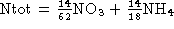. A background literal performing multiplication was introduced as well.

Since there were a lot of literals testing the value of Month roughly corresponding to the time of season change, we also defined background literals describing the seasons. This background knowledge was used in subsequent experiments and, particularly in experiments using the MDL pruning, it appeared very often in the induced models, while literals directly testing the value of Month appeared less frequently.

Experiment with Additional Attributes

Experiment with additional attributes resulted in an excellent (in experts opinion) model with the lowest error of all the models generated in this domain, which also incorporated newly derived attributes and a background knowledge literal defining autumn. Non-default values of parameters were: minimal number of examples MinNoExs=10 and maximal number of linear regression variables MaxLRVars=2.

 

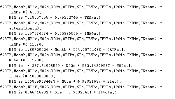
Figure 4: Model of biomass quantity in the Lake of Bled. BIM = maximal biomass quantity in the metalimnion of the east basin, e = epilimnion, m = metalimnion. Unused variables were removed from heads of the clauses for better readability. The model was generated in 17 minutes of CPU time on Sun SPARCstation 10.

We present the model in Figure 4, while the expert's comment on the model follows here.

• The first clause describes winter.
• The second clause describes the phase of biomass decomposition. This clause also makes use of one of the newly added attributes.
• The third clause describes spring conditions of the algal growth in months 2, 3, 4 (maybe 5). At this time the blue-green algae prevail. For them the limiting factor of growth is phosphorus (enough P implies plenty of algae). This comment was produced only after the expert took a closer look at the examples, covered by the clause.
• The fourth clause models the decomposition of biomass in both, epilimnion and metalimnion.
• The fifth clause covers some of the largest extremes in biomass quantity. Phosphorus was consumed by the algae. The quantity of NO₂ is minimal or zero. That shows the phase of algal growth (no decomposition, NH₄). Besides P the algae also consumed N. Term with Si shows the growth of Si algae.
• The last clause shows preparation of Si algae in early summer. At that time blue-green algae prevail which is indicated by both terms in the linear expression.

The course of events, indicated by the model, agrees with experts description of what is going on in the lake over one year: ``In epiliminion a spring algal bloom takes place in March/April, after which algae move into metalimnion, where the annual maximum occurs at the end of spring or beginning of summer.

In summary, the expert's opinion is that the induced models describe the growth of algae quite well. The use of linear regression largely increased the expressive power of the models, since it provided the expert with additional information about the behavior of the biomass in a selected region of the attribute space. The expert was also very satisfied with the usage of additional attributes. Newly induced background literals defining seasons helped in better comprehensibility of the induced models, but they did not improve the performance of the models on the learning set.

References

1. A. Karalic, I. Bratko: First Order Regression. Machine Learning, Kluwer (in press).
2. B. Kompare, S. Dzeroski, A. Karalic, I. Bratko, M. Sisko, S.E. Jorgensen. Using machine learning techniques in the construction of models, Part III: Learning systems with regression. Submitted to Ecological Modelling, 1996
3. B. Kompare and M. Rismal. Modelling the Lake of Bled. ISEM's Eighth International Conference on the Stat-Of-The-Art in Ecological Modelling. Kiel, Germany, 1992.

back to index